Traffic Model

These are the jupyter-notebook code we present here and the complete python code for finding other properties.

• jupyter-notebook code
• python code

This page will introduce how to write code to simulate traffic flow. Assume that each vehicle is only a point in the simulation. Two crucial pieces of information that we care about are these vehicles' positions and velocities. To simulate these values, we need to import two useful packages in python: numpy and matplotlib. Numpy is a very useful package providing quick and precise scientific simulation, and Matplotlib is a useful package to visualize the data from your simulation. To be more specific, we do not import all Matplotlib packages. We only import the class pyplot, which is enough to process data, in Matplotlib. Since typing all package names whenever we need the package wastes a lot of time, we can give them nicknames to simplify them. Common nicknames for numpy and matplotlib.pyplot are np and plt, respectively.

import numpy as np
import matplotlib.pyplot as plt

Next, we define two variables: "totalcarn" and "length," which specify the number of vehicles on the track and the length of the track. In this case, the total vehicle number is defined as 32. Since the track we are investigating is circular, the radius can be quickly found and defined as variable "r." Moreover, because we plan to investigate the condition that a steady flow transits to a traffic jam, the initial condition will be set such that the angular differences between vehicles are the same. The constant angular difference is defined as "alpha." The variable background, fig, and ax are used for plotting background tracks and plotting.

totalcarn = 2**5
length = totalcarn*6
r = length/(2*np.pi)
alpha = 2*np.pi/totalcarn 
background = np.linspace(0, 2*np.pi, 100)
fig, ax = plt.subplots()

Now, since the acceleration of each vehicle depends on the inter-vehicle distance, we define a function for calculating it. The first step is to find the difference of positions that are stored in numpy array. Thus, we call "diff" function, which returns the value of [function[1]-function[0], function[2]-function[1], ... ]. However, the difference will not calculate the inter-vehicle distance between the final vehicle and the first one. Therefore, we need to expand it into the difference array.

def deltaxfunction(length, function):    

    delta = np.diff(function)
    delta = np.append(delta, function[0]+length-function[-1])
  
    return delta

Finally, we can start our simulations. The first few lines are used for defining the initial condition, which is the positions of vehicles that are equally distributed on the track and add a small perturbation. The equally distributed position is initially defined as "x" and the perturbation we used here is a sin function. We only need to notice that the perturbation should not be too large since we applied linear perturbation in our analysis. The initial velocity is set to be ideal, which means all drivers drive with their desired velocity, and since the vehicles are initially equally distributed, all velocities are the same. Theoretically, the jamming transition of the system is when $$ \tau = \frac{1}{2}\left(\frac{dv_{\text{opt}}(\Delta x)}{d\Delta x}\right)\Bigg|_{\Delta x = L/N} \equiv \frac{1}{\text{sense}}. $$ Thus, the ideal sense is defined, and everyone can tune the coefficient such that the sense is different from its ideal value.

During the simulation, we apply two simulation methods. The first one is used for finding the optimal iteration time step. The reason for using this method is that using a fixed time step might cause a collision between two vehicles when they are too close to each other. Therefore, in each iteration, we use 0.01 times the minimal value of inter-vehicle distances divided by their velocities as the iteration time step. By doing so, all vehicles can not collide with each other. The other simulation method is the common fourth-order Runge-Kutta (See Wikipedia for detail).

x = np.linspace(0, length, totalcarn, endpoint=False)
idealdeltax = x[1]-x[0]
v = np.full(totalcarn, np.tanh(idealdeltax-2)+np.tanh(2))
theorysense = 2*(1/np.cosh(length/totalcarn-2)**2)/(np.cos(alpha/2)**2)
simulationtime = 0
coefficient = -0.01
sense = theorysense + coefficient
perturbe = 0.001*np.sin(x)

x = x+perturbe
while simulationtime < 600000:

    deltax = deltaxfunction(length, x)
    dt = np.min(deltax/v)*0.01
    
    k1x = v
    k1v = sense * (np.tanh(deltax-2)+np.tanh(2) - v)
    k2x = v + (dt * k1v * 0.5)
    k2v = sense * (np.tanh(deltaxfunction(length, x+(0.5*dt*k1x))-2)+np.tanh(2) - (v+(0.5*dt*k1v)))
    k3x = v + (dt * k2v * 0.5)
    k3v = sense * (np.tanh(deltaxfunction(length, x+(0.5*dt*k2x))-2)+np.tanh(2) - (v+(0.5*dt*k2v)))
    k4x = v + (dt * k3v)
    k4v = sense * (np.tanh(deltaxfunction(length, x+(dt*k3x))-2)+np.tanh(2) - (v+(dt*k3v)))

    x += dt*(k1x+2*k2x+2*k3x+k4x)/6
    v += dt*(k1v+2*k2v+2*k3v+k4v)/6
    
    simulationtime += 1

Now, we can plot out our results by matplotlib. The first line is the plot for the background track. The other is the plot for all vehicles.

ax.plot(r*np.cos(background), r*np.sin(background), 'b-')
ax.plot(r*np.cos(theta), r*np.sin(theta), color='r', marker = 'o', linestyle='None')
plt.show()

The final result is shown as the following figure

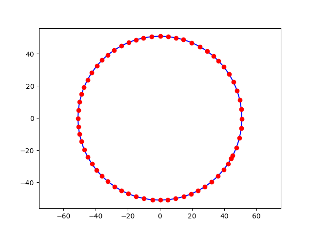
Apparently, a traffic jam occurs at the southeast of the figure. This occurrence is because the sensitivity is too small, which means drivers need more time to react. This result implies that Bando's model can qualitatively reproduce the jamming transition of a traffic system with an extremely simple model, and one crucial factor for jamming transition is human reaction time. If interested, you are encouraged to save figures at different time steps and make a movie to see how a traffic jam happens. The final result is shown in the following video. Interestingly, you can see some oscillation before jamming. That is because drivers try to accelerate and constantly decelerate at that time, and the reason is that, again, the reaction is too long, such that all drives do not have enough time to react.