Traffic Model

These are the jupyter-notebook code we present here and the complete python code for finding other properties.

• jupyter-notebook code
• python code

Based on the code we wrote in Bando's model, we only need to slightly change our simulations. First of all, the equilibrium condition will occur when $$ w_n \Delta x_n = \text{Const} $$ with the constraint $$ \sum_n \Delta x_n = L, $$ where L is the track length. Therefore, we define a function to find the equilibrium state. To calculate, we call the constat "A," and thus $\Delta x_n = A/w_n$. Therefore, $$ A = \frac{L}{\sum_n 1/w_n}. $$ We can use this to find out the initial position of all vehicles.

def fixed_solution(length, totalcarn, w):

    denominator = 0
    for i in w:
        denominator += 1/i
    A = length / denominator
    delta_x_i = A/w

    initial_position = [0]
    for i in range(0, len(delta_x_i)-1):
        initial_position.append(initial_position[len(initial_position)-1]+delta_x_i[i])

    return np.array(initial_position)

Next, we define two variables: "totalcarn" and "length," which specify the number of vehicles on the track and the length of the track. In this case, the total vehicle number is defined as 32. Since the track we are investigating is circular, the radius can be quickly found and defined as variable "r." Moreover, because we plan to investigate the condition that a steady flow transits to a traffic jam, the initial condition will be set such that the angular differences between vehicles are the same. The constant angular difference is defined as "alpha." The variable background, fig, and ax are used for plotting background tracks and plotting.

totalcarn = 2**5
length = totalcarn*6
r = length/(2*np.pi)
alpha = 2*np.pi/totalcarn 
background = np.linspace(0, 2*np.pi, 100)
fig, ax = plt.subplots()

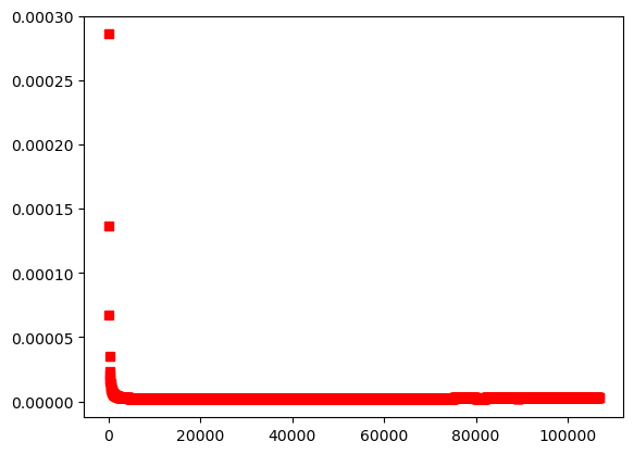
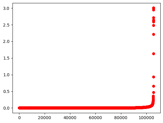
Now, we can set the initial condition and simulate. In this case, I denote the maximum value of the difference between current persection distance and the initial perception distance. Apparently, if a jam will occur in a traffic system, the difference will become larger. By comparing the result of identical drivers and drivers with individual difference, we can observe that the introduction of individual difference suppress tha jamming transition! See Fig. 1 for the case of drivers with individual difference, Fig 2. for the case of identical driver.

w = np.random.normal(1, 0.1, totalcarn) # w = np.random.normal(1, 0, totalcarn) for identical drivers
x = fixed_solution(length, totalcarn, w)
idealdeltax = w[0]*(x[1]-x[0])

v = np.full(totalcarn, np.tanh(idealdeltax-2)+np.tanh(2))
theorysense = 2*(1/np.cosh(length/totalcarn-2)**2)/(np.cos(alpha/2)**2)
coefficient = -0.02
sense = theorysense + coefficient
perturbe = 0.001*np.sin(x)

x = x+perturbe
simulationtime = 0
denote = []
denotetime = []
totaltime = 0
while simulationtime < 2162237:

    deltax = deltaxfunction(length, x)
    dt = np.min(deltax/v)*0.01

    k1x = v
    k1v = sense * (np.tanh(w*deltax-2)+np.tanh(2) - v)
    k2x = v + (dt * k1v * 0.5)
    k2v = sense * (np.tanh(w*deltaxfunction(length, x+(0.5*dt*k1x))-2)+np.tanh(2) - (v+(0.5*dt*k1v)))
    k3x = v + (dt * k2v * 0.5)
    k3v = sense * (np.tanh(w*deltaxfunction(length, x+(0.5*dt*k2x))-2)+np.tanh(2) - (v+(0.5*dt*k2v)))
    k4x = v + (dt * k3v)
    k4v = sense * (np.tanh(w*deltaxfunction(length, x+(dt*k3x))-2)+np.tanh(2) - (v+(dt*k3v)))
    x += dt*(k1x+2*k2x+2*k3x+k4x)/6
    v += dt*(k1v+2*k2v+2*k3v+k4v)/6
    simulationtime += 1
    totaltime += dt
    
    
    if simulationtime % 1000 == 0 :
        print(simulationtime)
        delta = w*deltaxfunction(length, x)
        denote.append(max(abs(delta-idealdeltax)))
        denotetime.append(totaltime)
        

ax.plot(denotetime, denote, 'ro')